Welcome to my work
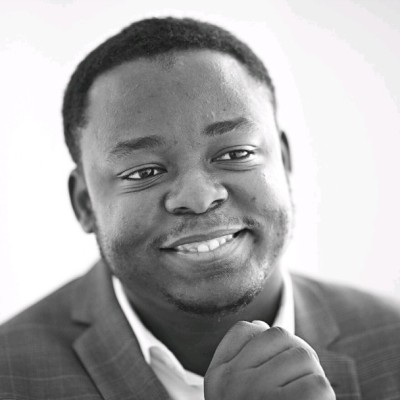
I'm Audric Dongfack. I work at the frontier of quantitative finance, applied mathematics, and artificial intelligence, exploring how rigorous mathematical models can unlock better decisions in complex, uncertain environments.
From interest-rate derivatives and stochastic optimization to machine learning, systematic investment research, and autonomous systems, my interests lie in translating sophisticated theory into computational solutions.
Here, I share my research, quantitative models, and interactive simulations – exploring ideas with the potential to shape the future of finance and intelligent technology.
Audric Dongfack
Strategy, Quantitative Finance & Machine Learning
I'm Audric Dongfack, a quantitative finance professional with an engineering master's degree from École Centrale Méditerranée and over five years of experience in the financial industry, including roles at BNP Paribas, Crédit Agricole, and Société Générale.
My interests lie at the intersection of quantitative finance, applied mathematics, artificial intelligence, and robotics. I'm particularly drawn to complex problems involving financial modelling, stochastic optimization, machine learning, and decision-making under uncertainty.
I believe in bridging mathematical theory and real-world applications, turning rigorous research into practical solutions that drive innovation and better decisions.
Photo credit: lightning storm over the ocean by bigwavephoto, Wikimedia Commons, CC BY-SA 4.0.
Problem
XVA desks and risk engines evaluate callable and path-dependent interest-rate products (Bermudan swaptions, callable range accruals, TARNs) millions of times a day: one price per market scenario, per counterparty, per time step. Each evaluation is itself a Monte Carlo or least-squares Monte Carlo run that takes seconds. A surrogate replaces the pricer by a fast function approximator over market states and contract parameters, trained offline on noisy Monte Carlo labels.
The difficulty is not speed but trust. A free-form regressor fitted to noisy prices oscillates, violates no-arbitrage relationships and produces unusable Greeks. The work is to build surrogates that satisfy the financial constraints by construction, so that both prices and sensitivities can be used in production.
Model
The underlying rates model is the one-factor Hull–White short-rate model, fitted to the initial curve through \(\theta(t)\):
\[ dr_t = \big(\theta(t) - a\,r_t\big)\,dt + \sigma\,dW_t, \qquad P(t,T) = A(t,T)\,e^{-B(t,T)\,r_t},\quad B(t,T) = \frac{1-e^{-a(T-t)}}{a}. \]
A payer swaption with expiry \(T\) on a swap with annuity \(A_0\) and forward swap rate \(S_0\) is priced under the annuity measure; with a normal (Bachelier) volatility \(\sigma_N\) implied by the model,
\[ V(K) = A_0\Big[(S_0-K)\,\Phi(d) + \sigma_N\sqrt{T}\,\varphi(d)\Big], \qquad d = \frac{S_0-K}{\sigma_N\sqrt{T}}. \]
Bermudan and callable products have no closed form: their value is the dynamic-programming recursion \(V_t = \max(\text{exercise}_t,\ \mathbb E_t[V_{t+1}])\), with continuation values estimated by regression on simulated paths (Longstaff–Schwartz). This is the slow pricer the surrogate must replace.
Surrogate under constraints
Let \(x = (r_0, a, \sigma, K, T, \dots)\) collect the market state and contract parameters, and \(\hat V_i\) be a noisy Monte Carlo label with standard error \(s/\sqrt{M}\) for \(M\) paths. The surrogate \(f_w\) minimizes a loss that mixes fit and shape penalties:
\[ \mathcal L(w) = \frac1N\sum_i \big(f_w(x_i)-\hat V_i\big)^2 + \lambda_1 \sum_i \big(\partial_K f_w(x_i)\big)_+^2 + \lambda_2 \sum_i \big(-\partial_{KK} f_w(x_i)\big)_+^2 + \lambda_3 \sum_i \big(\text{intrinsic}_i - f_w(x_i)\big)_+^2 . \]
The three penalties encode what a payer price must satisfy: decreasing in strike, convex in strike (the butterfly condition), and bounded below by the intrinsic value. In the strike direction the constraints can also be made hard by choosing the function class: any non-negative combination of hinge functions
\[ f(K) = \sum_{j=1}^{J} w_j\,(k_j - K)_+ ,\qquad w_j \ge 0, \]
is automatically decreasing and convex, and fitting it is a non-negative least-squares problem. The same idea scales to neural networks through input-convex architectures (Amos, Xu & Kolter), where convexity in selected inputs is guaranteed by non-negative weights and convex activations. A second benefit of constraints is that they act as a regularizer whose strength does not need to be tuned to the label noise: the noisier the Monte Carlo labels, the more the shape prior does.
Simulation
Everything below runs in your browser. Monte Carlo labels are real: each one averages \(M\) simulated terminal swap rates. The unconstrained surrogate is a degree-8 Chebyshev polynomial fitted by least squares; the constrained one is the hinge model above fitted by non-negative least squares. Timings are measured live.
Hull–White paths and a constrained swaption surrogate
2y × 5y payer swaption · prices in bp of notional
Short-rate paths r(t) with analytic mean and ±2σ band
Price vs strike: Monte Carlo labels, two surrogates, true price
constrained (convex, decreasing)unconstrained polynomialtrue Bachelier priceMC label ± 2 s.e.
RMSE vs true · constrained
–
RMSE vs true · unconstrained
–
Convexity violations · unconstrained
–
Surrogate time per price
–
What to look for: lower \(M\) makes labels noisier, and the polynomial starts to wiggle and to break convexity, while the constrained fit barely moves. Higher \(\sigma\) widens the price curve; higher \(a\) flattens the paths and lowers the implied normal volatility \(\sigma_N \approx \sigma\,B(0,5)/5\).
References
- Hull, J. & White, A. (1990). Pricing interest-rate-derivative securities. Review of Financial Studies.
- Longstaff, F. & Schwartz, E. (2001). Valuing American options by simulation. Review of Financial Studies.
- Amos, B., Xu, L. & Kolter, J. Z. (2017). Input convex neural networks. ICML.
- Glau, K. & Wunderlich, L. (2022). The deep parametric PDE method and applications to option pricing. Applied Mathematics and Computation.
Problem
Stress tests, reverse stress tests and model validation need joint scenarios of the yield curve and the volatility surface that are extreme yet coherent: a curve inversion that comes with the volatility spike that historically accompanies it, not a parallel +200 bp shock with volatility left untouched. Thirty years of daily history is roughly 7,500 observations and contains a handful of genuine tail events, which is not enough to estimate joint tails directly.
The approach is to learn the joint distribution \(p(x)\) of \(x = (\text{curve}, \text{vol surface}) \in \mathbb R^d\) with a generative model, and to sample its tails on purpose by controlling the latent space rather than hoping that random sampling will reach them.
Model
A variational autoencoder learns an encoder \(q_\phi(z\mid x)\) and a decoder \(p_\theta(x\mid z)\) with a latent prior \(z\sim\mathcal N(0,I_{d_z})\), by maximizing the evidence lower bound
\[ \mathcal L(\theta,\phi) = \mathbb E_{q_\phi(z\mid x)}\big[\log p_\theta(x\mid z)\big] - \mathrm{KL}\big(q_\phi(z\mid x)\,\|\,\mathcal N(0,I)\big). \]
Extreme scenarios are produced by changing how \(z\) is sampled while keeping the decoder fixed:
- Temperature. \(z\sim\mathcal N(0,\tau^2 I)\) with \(\tau>1\) stretches the prior and pushes samples outward.
- Radius conditioning. Sample on the shell \(\|z\|^2 \ge r_\alpha^2\) with \(r_\alpha^2 = \chi^2_{d_z}(\alpha)\), which targets the \((1-\alpha)\) most unlikely region of the latent space directly.
- Guidance. With a score-based (diffusion) model, \(dx = -\tfrac12\beta(t)x\,dt + \sqrt{\beta(t)}\,dW\), the reverse process can be steered toward a stress label with classifier-free guidance.
Validation uses extreme-value theory. Exceedances \(y = X-u\) over a high threshold \(u\) follow a generalized Pareto distribution,
\[ F_u(y) \approx 1 - \Big(1 + \xi\,\frac{y}{\beta}\Big)^{-1/\xi}, \]
and the tail index \(\xi\) estimated on generated scenarios must match the one estimated on history. Two further checks: the first three principal components of generated curves must explain the same variance share as in history (level, slope, curvature above 95%), and every scenario must pass no-arbitrage filters (finite implied forwards, positive volatilities, calendar and butterfly conditions on the surface).
Simulation
The decoder below stands in for a trained network: three latent factors map to the level, slope and curvature of a Nelson–Siegel curve, and a volatility level coupled to the latent so that inverted or very high curves come with high volatility. Drag the point in the latent pad to steer one scenario; the temperature slider stretches the prior for all 400 samples.
Latent sampling of yield-curve and volatility scenarios
400 samples · tail = outside the 99% latent shell
Generated yield curves (tail scenarios highlighted, selected scenario bold)
Latent pad z₁ × z₂ (rings: 90% and 99% shells)
10y yield across samples, with a GPD fitted above the 95th percentile
Normal volatility surface of the selected scenario (bp)
Selected: 2y / 10y / vol
–
What to look for: at \(\tau = 1\) roughly 1% of samples land in the tail shell. Raising \(\tau\) multiplies that share and also raises the fitted tail index \(\xi\), which is exactly the quantity you compare with history to decide whether the generator exaggerates or understates the tails. Dragging the pad to the lower-left produces low, inverted curves with high volatility: the regime of a flight-to-quality episode.
References
- Kingma, D. P. & Welling, M. (2014). Auto-encoding variational Bayes. ICLR.
- Song, Y. et al. (2021). Score-based generative modeling through stochastic differential equations. ICLR.
- Embrechts, P., Klüppelberg, C. & Mikosch, T. (1997). Modelling Extremal Events. Springer.
- Nelson, C. R. & Siegel, A. F. (1987). Parsimonious modeling of yield curves. Journal of Business.
Problem
Mean–variance portfolios are notoriously unstable: small estimation errors in the expected returns \(\hat\mu\) and the covariance \(\hat\Sigma\) turn into large swings in the weights and poor out-of-sample performance. Distributionally robust optimization (DRO) replaces the single estimated distribution by an ambiguity set of distributions close to it and optimizes against the worst member of that set. Optimal transport gives the right notion of closeness: the Wasserstein distance measures how much probability mass must be moved, and how far, to turn one distribution into another.
Model
For two distributions \(P, Q\) on \(\mathbb R^n\), the \(p\)-Wasserstein distance is the cheapest coupling
\[ W_p(P,Q) = \Big( \inf_{\pi\in\Pi(P,Q)} \int \|x-y\|^p\, d\pi(x,y) \Big)^{1/p}, \]
where \(\Pi(P,Q)\) is the set of joint distributions with marginals \(P\) and \(Q\). The robust portfolio problem over the simplex \(\Delta\) with a ball of radius \(\varepsilon\) around the empirical distribution \(\hat P_N\) reads
\[ \min_{w\in\Delta}\ \sup_{Q:\ W_1(Q,\hat P_N)\le\varepsilon}\ \mathbb E_Q\big[-w^\top\xi\big] + \frac{\gamma}{2}\, w^\top\hat\Sigma w . \]
For a loss that is Lipschitz in \(\xi\), the inner supremum has a closed form (Mohajerin Esfahani & Kuhn, 2018): the worst case adds \(\varepsilon\) times the Lipschitz constant. With \(\ell(\xi) = -w^\top\xi\) that constant is the dual norm \(\|w\|_*\), so the robust problem becomes a regularized Markowitz problem,
\[ \min_{w\in\Delta}\ -w^\top\hat\mu + \varepsilon\,\|w\|_2 + \frac{\gamma}{2}\, w^\top\hat\Sigma w . \]
The ambiguity radius \(\varepsilon\) is not a free parameter: it can be calibrated as the transport distance between market regimes, computed on samples with the entropic (Sinkhorn) algorithm
\[ \pi^\eta = \arg\min_{\pi\in\Pi(a,b)} \langle C,\pi\rangle - \eta\,H(\pi), \qquad \pi^\eta = \mathrm{diag}(u)\,K\,\mathrm{diag}(v),\quad K = e^{-C/\eta}, \]
with the scalings \(u \leftarrow a / (Kv)\), \(v \leftarrow b / (K^\top u)\) iterated to convergence. Each iteration is two matrix–vector products, which is what makes transport usable on thousands of return observations.
Simulation
Left: daily returns of two assets in a calm regime and in a stress regime (60 observations each). The Sinkhorn iterations resolve the coupling live; the line opacity is the transported mass. Right: the robust portfolio on five assets as the ambiguity radius grows, solved by projected gradient on the simplex.
Transport between regimes and the robust weight path
5 assets · annualized μ̂ and Σ̂ · γ = 0.05
Entropic transport plan: calm regime → stress regime (daily returns, %)
Robust weights as a function of ε (marker = current ε)
Sinkhorn W₂ calm → stress
–
Iterations · marginal error
–
Effective number of assets
–
What to look for: at \(\varepsilon = 0\) the weights are the nominal Markowitz solution, concentrated in the assets with the highest estimated return. As \(\varepsilon\) grows the \(\|w\|_2\) term pulls the portfolio toward equal weights and the effective number of assets rises. The transport distance between regimes on the left gives a data-driven scale for \(\varepsilon\): a radius smaller than that distance does not protect against a regime change.
References
- Mohajerin Esfahani, P. & Kuhn, D. (2018). Data-driven distributionally robust optimization using the Wasserstein metric. Mathematical Programming.
- Cuturi, M. (2013). Sinkhorn distances: lightspeed computation of optimal transport. NeurIPS.
- Peyré, G. & Cuturi, M. (2019). Computational optimal transport. Foundations and Trends in Machine Learning.
- Blanchet, J., Chen, L. & Zhou, X. Y. (2022). Distributionally robust mean-variance portfolio selection with Wasserstein distances. Management Science.
Problem
A trader must liquidate \(X\) shares over a horizon \([0,T]\). Selling fast moves the price against them (market impact); selling slowly exposes the remaining inventory to price risk. The problem is to choose the trading rate \(v_t\) that balances expected cost against risk, first in the classical linear-impact model where it has a closed form, then in realistic settings where it does not and must be learned.
Model: Almgren–Chriss
The unaffected price is arithmetic Brownian, permanent impact is linear in the trading rate, and the execution price carries a temporary impact:
\[ dS_t = \sigma\,dW_t - \gamma\,v_t\,dt, \qquad \tilde S_t = S_t - \eta\,v_t, \qquad x_t = X - \int_0^t v_s\,ds . \]
The implementation shortfall \(C\) (cost relative to the arrival price) has mean and variance
\[ \mathbb E[C] = \tfrac{\gamma}{2}X^2 + \eta\int_0^T v_t^2\,dt, \qquad \mathrm{Var}[C] = \sigma^2\int_0^T x_t^2\,dt , \]
and minimizing \(\mathbb E[C] + \lambda\,\mathrm{Var}[C]\) is a deterministic calculus-of-variations problem whose solution is the hyperbolic-sine trajectory
\[ x^*_t = X\,\frac{\sinh\big(\kappa (T-t)\big)}{\sinh(\kappa T)}, \qquad \kappa = \sqrt{\frac{\lambda\sigma^2}{\eta}} . \]
The same answer comes out of the dynamic-programming route. With value function \(V(t,x)\) the Hamilton–Jacobi–Bellman equation is
\[ \partial_t V + \min_v\Big\{ \eta v^2 + \lambda\sigma^2 x^2 - v\,\partial_x V \Big\} = 0,\qquad V(T,x) = +\infty\ \text{for } x\neq 0, \]
whose minimizer \(v^* = \partial_x V / (2\eta)\) with a quadratic ansatz \(V = h(t)x^2\) gives a Riccati equation for \(h\) and the trajectory above.
Reinforcement learning
Once impact is nonlinear (\(\eta v^{3/2}\) is the empirical norm), stochastic, or depends on the state of the order book, the HJB equation has no closed form and the problem is naturally an MDP: state \(s_k = (t_k, q_k, S_k, \text{book features})\), action \(v_k\), reward
\[ r_k = -\big(\text{cost increment}_k\big) - \lambda\,\sigma^2 q_k^2\,\Delta t, \qquad Q(s,a) \leftarrow Q(s,a) + \alpha\Big[r + \max_{a'}Q(s',a') - Q(s,a)\Big]. \]
Tabular Q-learning is enough for a small discretized problem and makes the learned policy inspectable; with order-book features one moves to actor–critic methods (PPO, DDPG) with the Almgren–Chriss schedule as a baseline and as a sanity check.
Simulation
The agent below is a tabular Q-learner on 20 time steps and 20 inventory units, trained live on the linear-impact model so that its schedule can be compared with the closed form. Costs are in currency units per share of the parent order; 400 Monte Carlo episodes per strategy build the histograms.
TWAP, Almgren–Chriss and a Q-learning agent
X = 1 (normalized) · T = 1 day · 20 steps · σ = 1.5 per √day
Distribution of implementation shortfall (400 episodes each)
TWAPAlmgren–ChrissQ-learning (greedy policy)
Learning curve: mean episode cost (moving average)
Almgren–Chriss · mean ± sd
–
What to look for: TWAP has the lowest expected cost but the widest distribution. Raising \(\lambda\) makes the closed-form schedule front-loaded (larger \(\kappa\)), trading expected cost for a narrower distribution. The Q-learner, trained on nothing but sampled rewards, recovers a schedule close to the closed form, which is the test that justifies using it where no closed form exists.
References
- Almgren, R. & Chriss, N. (2001). Optimal execution of portfolio transactions. Journal of Risk.
- Cartea, Á., Jaimungal, S. & Penalva, J. (2015). Algorithmic and High-Frequency Trading. Cambridge University Press.
- Nevmyvaka, Y., Feng, Y. & Kearns, M. (2006). Reinforcement learning for optimized trade execution. ICML.
- Ning, B., Lin, F. H. T. & Jaimungal, S. (2021). Double deep Q-learning for optimal execution. Applied Mathematical Finance.
Problem
A surveillance multirotor must hold a stable camera over a patrol route for as long as possible, in wind, while carrying a gimbal and a transmitter. Three mechanical questions decide the design: how the rotors' thrust and torque turn into rigid-body motion, how a controller keeps the vehicle on its path when gusts push it off, and how much flight time a given battery, airframe mass and rotor disc area can buy.
Model: rigid-body dynamics
With position \(\mathbf p\) in the world frame, rotation \(R\) from body to world, angular velocity \(\boldsymbol\omega\) in the body frame and inertia \(J\), Newton–Euler gives
\[ m\,\ddot{\mathbf p} = m\mathbf g + R\,\mathbf e_3 \sum_{i=1}^4 T_i + \mathbf F_d, \qquad J\,\dot{\boldsymbol\omega} = \boldsymbol\tau - \boldsymbol\omega\times J\boldsymbol\omega, \]
where each rotor produces thrust and reaction torque proportional to the square of its speed, \(T_i = k_T\,\Omega_i^2\) and \(Q_i = k_Q\,\Omega_i^2\). For an X-configuration with arm length \(\ell\) the mixer maps rotor speeds to the collective thrust and the three body torques:
\[ \begin{pmatrix} T \\ \tau_\phi \\ \tau_\theta \\ \tau_\psi \end{pmatrix} = \begin{pmatrix} k_T & k_T & k_T & k_T \\ -\tfrac{\ell k_T}{\sqrt2} & \tfrac{\ell k_T}{\sqrt2} & \tfrac{\ell k_T}{\sqrt2} & -\tfrac{\ell k_T}{\sqrt2} \\ \tfrac{\ell k_T}{\sqrt2} & -\tfrac{\ell k_T}{\sqrt2} & \tfrac{\ell k_T}{\sqrt2} & -\tfrac{\ell k_T}{\sqrt2} \\ k_Q & k_Q & -k_Q & -k_Q \end{pmatrix} \begin{pmatrix} \Omega_1^2 \\ \Omega_2^2 \\ \Omega_3^2 \\ \Omega_4^2 \end{pmatrix}. \]
In the vertical plane the model reduces to three degrees of freedom, which is enough to study pitch control and gust rejection:
\[ \ddot x = -\frac{T}{m}\sin\theta - \frac{c}{m}\dot x + \frac{F_w}{m},\qquad \ddot z = \frac{T}{m}\cos\theta - g - \frac{c}{m}\dot z,\qquad \ddot\theta = \frac{\tau}{I_{yy}} . \]
Control
The controller is cascaded. An outer position loop turns the tracking error into a desired acceleration, \(\mathbf a_d = k_p(\mathbf p_d - \mathbf p) - k_d\,\dot{\mathbf p}\); the desired tilt and collective thrust follow from the geometry, \(\theta_d = -\arctan\big(a_{x,d}/(a_{z,d}+g)\big)\) and \(T = m\,(a_{z,d}+g)/\cos\theta\). A faster inner attitude loop produces the torque \(\tau = I_{yy}\big(k_{p\theta}(\theta_d-\theta) - k_{d\theta}\dot\theta\big)\). The inner loop must be several times faster than the outer one, which is why the attitude gains are an order of magnitude larger.
Endurance
Momentum theory gives the ideal hover power from thrust, air density and total rotor disc area \(A\); real rotors and motors are rated by a figure of merit \(\mathrm{FM}\) and an electrical efficiency \(\eta_m\):
\[ P_{\text{hover}} = \frac{(mg)^{3/2}}{\sqrt{2\rho A}\;\mathrm{FM}\;\eta_m}, \qquad t_{\text{flight}} = \frac{\eta_b\,E_{\text{batt}}}{P_{\text{hover}}} . \]
Because power grows as mass to the \(3/2\), every gram of payload costs more than the previous one, and because the battery is part of the mass, there is an optimal battery size beyond which more cells reduce flight time. For the camera, the ground sample distance \(\mathrm{GSD} = p\,h/f\) (pixel pitch \(p\), altitude \(h\), focal length \(f\)) sets the altitude at which a target of given size is still identifiable.
Simulation
A planar quadrotor patrols five waypoints at a set altitude with the cascaded controller above, integrated at 240 Hz. The gust button applies a 0.6 s horizontal force; light turbulence is always present. The endurance panel evaluates the momentum-theory formula for a four-rotor airframe.
Patrol flight with gust rejection, and endurance vs payload
planar model · ℓ = 0.25 m · c = 0.15 N·s/m · 240 Hz
Flight (side view): thrust arrows scale with rotor thrust, cone = camera footprint
Pitch θ (°) and altitude error (m), last 10 s
Endurance vs added payload (momentum theory, FM = 0.70, η_m = 0.85, 80% usable battery)
Endurance (no extra payload)
–
What to look for: a heavier airframe tilts less for the same gust but needs proportionally more thrust and loses endurance quickly. Lowering the attitude gain below about 15 makes the inner loop too slow for the outer loop and the vehicle starts to oscillate, which is the cascade-separation rule made visible. In the endurance panel, larger rotors lower the disc loading and raise flight time at every payload.
References
- Mahony, R., Kumar, V. & Corke, P. (2012). Multirotor aerial vehicles: modeling, estimation, and control of quadrotor. IEEE Robotics & Automation Magazine.
- Leishman, J. G. (2006). Principles of Helicopter Aerodynamics. Cambridge University Press.
- Mellinger, D. & Kumar, V. (2011). Minimum snap trajectory generation and control for quadrotors. ICRA.
- Beard, R. W. & McLain, T. W. (2012). Small Unmanned Aircraft: Theory and Practice. Princeton University Press.